Arrhenius Integrals, IR Lasers, and Cooking Proteins
Introduction
May 2016, Munich. I had just joined NanoTemper Technologies as a Bioanalytics Scientist. If you aren’t familiar with NanoTemper, they build high-end biophysical instruments. At the time, their newest platform was the Prometheus — a machine that performed nanoDSF (Differential Scanning Fluorimetry) for helping develop new medicines.
Developing antibody drugs is hard; even when you finally invent a new ‘cancer cure’, will it still be 98% monomeric and active after your miracle monoclonal antibody has sat in a glass vial at 4°C for two years, or will it have clumped into a useless, immunogenic aggregate, a bit like profoundly expensive sour milk?
Formulation scientists were obsessed with a single metric: the $T_m$ (melting temperature). This is where Nanotemper’s Prometheus comes in. The concept behind nanoDSF is elegant: you suck a few microliters of protein solution into a glass capillary, heat it up, and hit it with UV light. As the protein unfolds, its interior tryptophan residues are exposed to the solvent, which shifts their intrinsic fluorescence emission (measured as a ratio of 350 nm / 330 nm). It was vastly higher throughput and required a fraction of the sample volume compared to traditional Differential Scanning Calorimetry (DSC).
But there was a problem with how the biopharma industry was using it. They were treating this incredibly sophisticated optical instrument like a glorified meat thermometer.
The standard data processing pipeline was to take the raw sigmoidal fluorescence trace, slap a smoothing filter on it (Savitzky-Golay, spline, whatever), and take the first derivative to find the peak. If you had a complex multi-domain protein like an IgG antibody, you took the second derivative to find the zero-crossings. The logic was beautifully simple and fundamentally flawed: Higher $\ T_m$ = Better Drug. If your antibody melted at 65°C, it went in the bin. If it melted at 75°C, you moved it to clinical trials.
Mathematically, differentiating noisy data violently amplifies the noise. We were deliberately destroying our own signal resolution. Furthermore, biophysically, the first derivative of a protein melt is inherently asymmetric due to the Boltzmann distribution of energy states.
I decided we needed to ditch the derivative entirely. We needed to fit the raw trace analytically using the best thermodynamic models available at the time.
Here is the story of the math used built to do it, the infrared laser hacks to test it, and now looking back from a decade later, how the limits of those early models perfectly predicted the next decade of biophysical hardware.
Part 1: Brute-Forcing the Arrhenius Integral
In 2016, the most pragmatic way to model thermal denaturation in a high-throughput setting was as a purely kinetic, two-state irreversible process (Native $\to$ Denatured). The transition rate $k$ follows the standard Arrhenius equation:
\[k = A e^{-\frac{E_a}{RT}}\]To figure out the total amount of denatured protein ($FD$, Fractional Denaturation) generated during a constant-rate temperature ramp ($B$, in K/s), you have to integrate over temperature:
\[FD = 1 - \exp\left(-\frac{A}{B} \int_{T_0}^{T_{end}} e^{-\frac{E_a}{RT}} dT\right)\]Here’s the brick wall: the Arrhenius integral has no exact analytical solution. You cannot integrate $e^{-1/T}$ using standard elementary functions. You can numerically integrate it, but doing that iteratively inside a fitting algorithm for 48 parallel capillaries is computationally miserable.
So, I dug into the applied math literature and implemented an analytical approximation by Cai and Liu1. It is an absolute monster of an equation, but it calculates the Arrhenius Integral ($AIX$) extremely fast:
\[AIX \approx \frac{R T^2 \left(0.99994 E_a + 0.2786 RT \ln\left(\frac{E_a}{RT}\right) + 0.3672 RT\right) \, e^{-\frac{E_a}{RT}}}{E_a \left(E_a + 2.4383 RT + 0.2647 RT \ln\left(\frac{E_a}{RT}\right)\right)}\](Yes, those constants are real. Don’t ask.)
Because tryptophan fluorescence changes with temperature even when the protein isn’t melting, the baselines naturally slope. We modeled the raw signal $S$ with sloping baselines ($S_x = \alpha_x + \beta_x T$).
I wrote a Python script using a Levenberg-Marquardt minimizer to fit this analytical abomination directly to the raw 350/330nm ratio.
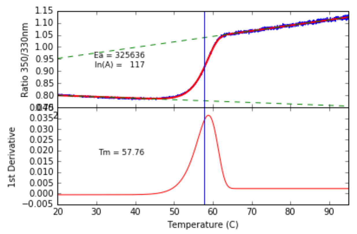
Fitting the Arrhenius integral to an alpha-Amylase melt.
It worked beautifully. We could pull the Activation Energy ($E_a$) and pre-exponential factor ($A$) out of a single trace without ever touching a derivative.
But as we pushed the model to its limits, the underlying complexity of protein folding started fighting back.
Part 2: The Ramp-Rate Anomaly & The Laser Hack
To prove that our single-trace Arrhenius integral was actually working, we needed a “ground truth” for the Activation Energy.
Traditionally, if you want to find the $E_a$ of a protein melt, you can’t just run one experiment. You have to run multiple thermal ramps at different heating speeds ($v$) and track how the $T_m$ shifts. A faster heating rate gives the protein less time to unfold, which artificially pushes the $T_m$ to a higher temperature.
This shift is mathematically governed by the Kissinger equation:
\[\frac{v}{T_m^2} = \frac{AR}{E_a} \, e^{-\frac{E_a}{R T_m}}\]If you plot $\ln(v / T_m^2)$ against $1/T_m$, you get a beautiful straight line. The slope of that line is exactly $-E_a / R$.
This multi-ramp method is incredibly robust. The problem? It is slow and eats up sample, because you have to run half a dozen different ramp rates to get one number. My analytical approximation was supposed to pull that exact same $E_a$ out of just a single curve.
But when I actually tested it across different heating rates (e.g., 1 K/min vs 5 K/min), I found a fascinating anomaly. The Activation Energy calculated from a single trace changed depending on how fast the machine was heating.
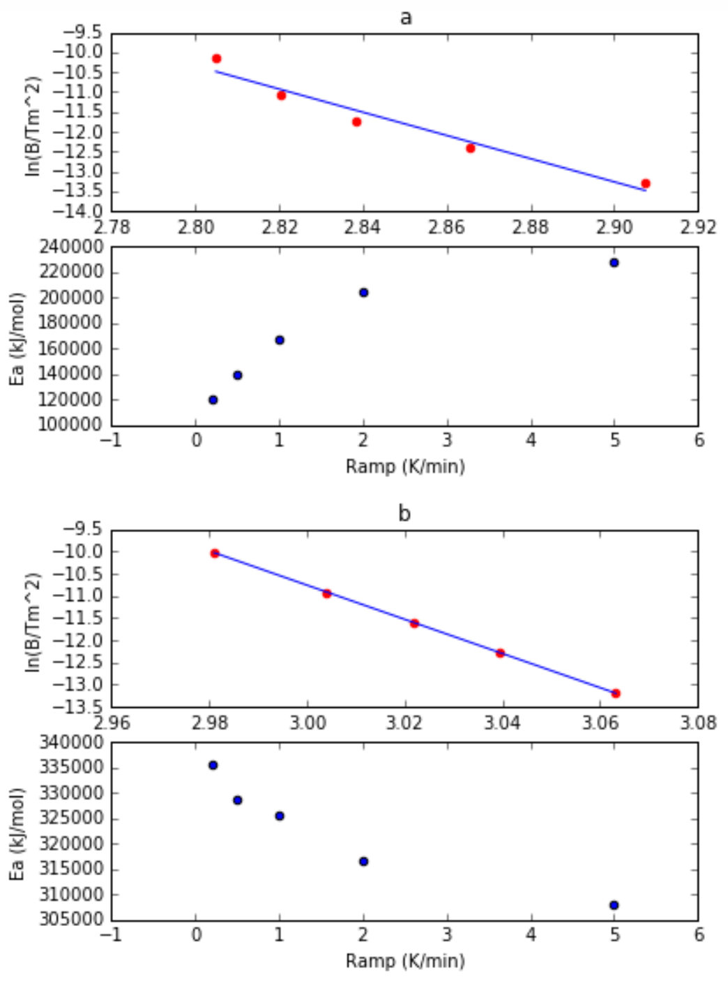
If $E_a$ is an intrinsic thermodynamic barrier, it shouldn’t care how fast the Prometheus is heating the sample. But it did. This wasn’t a bug in the code; it was our 2-state model reaching the absolute edge of its biophysical validity.
Real proteins don’t follow a simple 1-step irreversible melt ($N \to D$). They follow the Lumry-Eyring model:
\[N \rightleftharpoons U \longrightarrow D\]Unfolding is initially a reversible thermodynamic equilibrium ($N \rightleftharpoons U$). It only becomes irreversible when the unfolded protein clumps together and aggregates ($U \to D$). Furthermore, unfolding exposes a massive hydrophobic core to water, causing a huge spike in heat capacity ($\Delta C_p$). Because of $\Delta C_p$, the actual energy barrier to unfolding literally changes as the temperature rises!
At slow ramp rates, the protein hangs out in the transition zone for a long time. The reversible equilibrium fights against the 2nd-order aggregation kinetics, widening and skewing the shape of the curve. Our 1-step Arrhenius fit was trying to force a purely kinetic math onto a mixed-thermodynamic reality, and it was spitting out a skewed $E_a$.
But at fast ramp rates, we essentially outran the equilibrium. We pushed the protein into a regime of pure kinetic control. This is why the single-trace math suddenly snapped perfectly into place at higher speeds, asymptoting to match the theoretical multi-ramp Kissinger equations.
This highlighted a massive problem in biopharma. Formulation scientists were binning promising drug candidates just because they had a “low $T_m$.” But if that low-temperature melt was purely thermodynamic and reversible ($N \rightleftharpoons U$), the drug might be perfectly stable on a pharmacy shelf!
Standard thermal ramps couldn’t tell a reversible melt from an irreversible aggregation event. We needed a way to pulse the heat, check if the protein refolded, and do it fast enough to outrun the aggregation step.
We couldn’t use standard Peltier elements—they have too much thermal mass and cool down too slowly. So, I borrowed a toy from NanoTemper’s original instrument, the Monolith: a 1480 nm, 600 mW infrared laser. (actually, an engineering sample I found in the ‘random lasers’ box in the storeroom).
Water strongly absorbs at 1480 nm. By firing a collimated IR laser directly into the glass capillary, I could bypass the thermal mass entirely. I jury rigged a Raspberry Pi GPIO to pulse the laser to heat the sample with ~0.5°C resolution, running 200 discrete heat/cool cycles in just 20 minutes.
If the protein was reversible, we modeled the renaturation using the Van’t Hoff equation:
\[F(T) = \frac{F_N(T) + F_U(T) \exp\left( \frac{\Delta H_m (T-T_m)}{R T T_m} \right)}{1 + \exp\left( \frac{\Delta H_m (T-T_m)}{R T T_m} \right)}\]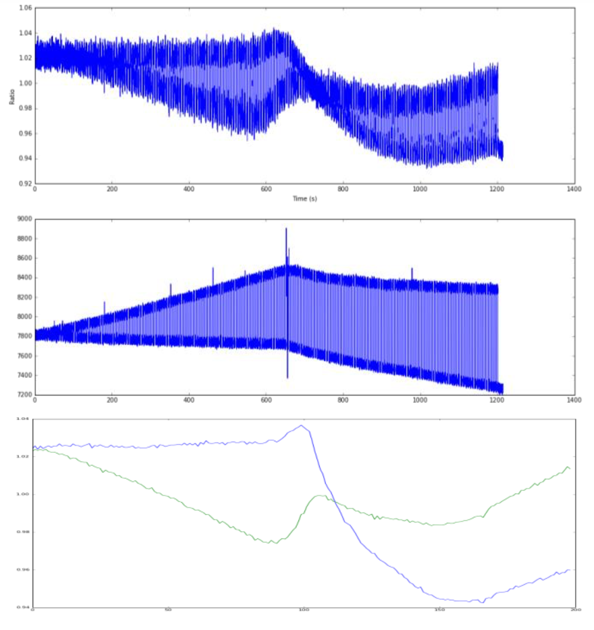
1480nm Laser pulsing. Each vertical blue line (yes, there are lots), is the sample being heated or cooled ridiculously fast. Why fast cooling? We are only heating a teeny tiny sample, at the focal point of the laser, and as soon as its turned off, the bulk solution around it cools and replaces the targetted zone. You can clearly see the reversible renaturation baseline (blue) pulling away from the forward melt curve (green) the moment irreversible aggregation kicks in.
We had successfully stress-tested the protein, catching the exact millisecond the reversible Lumry-Eyring equilibrium collapsed into an irreversible aggregate.
Part 3: Enter the AI (When the Math Gets Too Hard)
I don’t write Levenberg-Marquardt minimizers to fit Arrhenius equations anymore. These days, I spend my time spinning up Hopper GPUs and building AI models. But it is incredibly satisfying to see how the Deep Learning era has completely embraced what we were trying to do with those early nanoDSF curves.
If there is one thing I learned from trying to brute-force an analytical integral onto a Lumry-Eyring folding process, it’s that biology hates clean math. You can’t easily write a closed-form equation that perfectly accounts for reversible thermodynamics, irreversible aggregation kinetics, and a dynamic change in heat capacity ($\Delta C_p$) all happening simultaneously in a single capillary. There are simply too many overlapping variables.
So, the industry did what the tech world does when the math gets too hard: they stopped trying to write the equation and let an algorithm find the pattern.
Today, cutting-edge pharma doesn’t take the derivative. They don’t even extract the $T_m$. Instead, they take the entire raw time-series trace from modern multi-modal instruments like the Prometheus Panta—stacking the 350 nm fluorescence, the 330 nm fluorescence, and the light scattering radii into a multi-dimensional tensor.
They feed this raw, unadulterated data directly into 1D Convolutional Neural Networks (CNNs) and sequence models to do exactly what we set out to do: predict 2-year shelf life from a 1-hour temperature ramp.
When you peer into the attention heads of these models to see what features the AI is actually looking at, it isn’t looking at the inflection point. It is looking at the shape of the curve.
- Pre-transition baselines: The AI notices if the native baseline slopes upward slightly before the melt, representing conformational “breathing.”
- Asymmetry of the melt: The AI heavily weights the asymmetry of the unfolding curve—mathematically detecting the exact fight between the reversible equilibrium and the kinetic aggregation trap that my Arrhenius approximation was struggling to map.
- Scattering onset vs. unfolding: The AI looks at the precise millisecond the scattering signal ticks upward relative to the fluorescence shift, mapping the aggregation energy barrier dynamically.
It turns out, if you feed thousands of raw thermal denaturation curves into a neural network, the AI effectively derives the Lumry-Eyring model on its own. It figures out that protein unfolding is a multi-state thermodynamic and kinetic war, and it uses the raw curve shape to predict that an antibody will crash out of solution in 18 months.
Epilogue: A Funny Anecdote from the Literature
When you leave a field to pivot into a new one, you usually assume the internal tools you built gather dust on a server somewhere. I wrote those Python scripts, the Arrhenius integral approximations, and the 3-state models back in 2016, and then I eventually moved on to the world of AI.
But science has a funny way of leaving breadcrumbs.
Not too long ago, I was browsing the literature and stumbled across a 2021 PhD dissertation by Dr. Richard Weber from the Martin-Luther-Universität Halle-Wittenberg. It was part of a massive industrial collaboration between NanoTemper and the pharmaceutical giant Boehringer Ingelheim.
Their goal was the holy grail: figuring out which biophysical parameter actually correlates with long-term, real-world antibody stability (measured by Size Exclusion Chromatography over many months).
To do it, they had dug up the exact hardware modifications we had hacked together (dubbed the “NanoTemper Experimental Setup” or NES) and my old Python script with the Arrhenius fit function. They threw a massive library of therapeutic monoclonal antibodies (mAbs) at it to see what would happen.
Funny enough, the math held up.
The Thesis2 concluded that the Activation Energy ($E_a$) of the CH2-domain unfolding transition—extracted directly using our multi-ramp method and Arrhenius fits—was the absolute best predictor of actual thermal stability. It definitively outperformed the traditional $T_m$ and calorimetric enthalpy for predicting whether an antibody would aggregate on the shelf.
Furthermore3, they later published, showing exactly why we bothered building that 3-state model. Because therapeutic IgG antibodies have overlapping Fab, CH2, and CH3 transitions, taking the derivative turns the data into a noisy, unusable mess. Our analytical model cleanly deconvolved those overlapping curves, allowing the researchers to isolate the specific kinetic energy barrier of just the CH2 domain—which turned out to be the “weak link” triggering the irreversible aggregation.
It’s a pretty surreal feeling to realize that a Python script and some applied math I wrote to avoid doing calculus ended up helping a major pharma company prove that $T_m$ is an illusion.
Today, my toolkit looks very different. But whether you are wrestling with a Levenberg-Marquardt minimizer to fit a 3-state protein melt, or training a billion-parameter Transformer model on time-series tensor data, the lesson remains exactly the same:
Don’t destroy your data. Stop taking the derivative. The truth is always in the raw shape of the curve.
Refs
Kinetic analysis of nonisothermal solid-state reactions: Determination of the kinetic parameters by means of a nonlinear regression method
Journal of Mathematical Chemistry 44(2):551-558 (August 2008)
Authors: Junmeng Cai, Ronghou Liu
DOI:DOI:10.1007/s10910-007-9328-5 ↩︎Thermodynamic and kinetic unfolding characterization of therapeutic monoclonal antibodies using thermal analytics
Author: Richard Melien (née Weber)
Institution: Martin-Luther-Universität Halle-Wittenberg (in collaboration with Boehringer Ingelheim & NanoTemper)
Defense Date: June 11, 2021
Link to the full PDF via the Halle University library:PhD Thesis ↩︎“Expanding the toolbox for predictive parameters describing antibody stability considering thermodynamic and kinetic determinants”
Pharmaceutical Research (Dec 2021)
Authors: Michaela Blech, Richard Melien, Nuška Tschammer, Beate Presser, Dariush Hinderberger, Patrick Garidel.
DOI:10.1007/s11095-021-03120-x ↩︎
Enjoyed this deep-dive?
Get my next piece on AI hardware, biophysics, or random optimisation hacks delivered straight to your inbox.