The Cortical Ratio: A Thought Experiment on the 'Final' Size of AGI

No one knows how big AGI needs to be. The current consensus among the scaling-pilled crowd is “trillions of parameters and a nuclear power plant.” Maybe they’re right. But I spent years dissecting rat brains for my PhD, and the one thing neuroscience taught me is that biology is embarrassingly good at compression. What happens when we figure it out too?

There’s a quieter trend happening alongside the scaling race: for a given model size, capabilities are climbing fast. Qwen3.5-4B now matches or beats models 50× its size from just two years ago on standard benchmarks (yes, benchmarks are flawed, but the trajectory is real). Distillation keeps working better than it should. Small, purpose-built models keep eating tasks that were supposed to require frontier scale.

This got me thinking. We already have narrow AI systems that match or exceed human performance on specific sensory tasks (hearing, vision) and we know roughly how many parameters they needed to get there. We also know, from a century of neuroanatomy, roughly how the human brain allocates its computational budget across different functions.

Can we use the known cost of the “digital ear” and the “digital eye” as anchors, and then scale up to the “digital mind” using biological ratios?

This is a Fermi estimation. It will be wrong. The question is whether it’s usefully wrong.

---

The Anchors

The idea here is simple. Find tasks where silicon has caught up with biology, note how many parameters it took, and use those as reference points. I’m looking for compute saturation: the point where throwing more parameters at a specific task stops helping, because the task is effectively solved.

The Digital Ear

NVIDIA’s Canary-1B (v2) handles multilingual ASR and translation across 25+ languages at near-SOTA accuracy. One billion parameters. Runs in real-time on a Raspberry Pi 5 (I will post about this later).

Now, ASR is obviously not the full auditory cortex. Humans do source separation, spatial localisation, prosody decoding, musical perception, and a dozen other things beyond “convert pressure wave to text.” But transcription is the core transform: the fundamental signal-to-symbol conversion, and that’s the part that maps most directly onto what a model actually does.

Anchor 1: ~1B parameters for the core auditory transform.

The Digital Eye

Similar story for vision. The dense backbones of current video understanding models (SigLIP, InternViT, and friends), hit their stride somewhere in the 3–5B parameter range for core visual understanding: object permanence, occlusion, basic scene physics.

Again, not the full visual cortex. No mental rotation, no visual imagination, no dreaming. It’s the feedforward perceptual pipeline: pixels in, scene graph out.

Anchor 2: ~3.5B parameters (geometric mean) for core visual processing.

Are These Anchors Any Good?

Honestly? They’re rough. Mapping “human sensory cortex” to “neural network that does a similar task” is full of holes. The architectures are completely different. The representations are definitely different. We’re comparing a spiking recurrent biological circuit running on 20 watts to a feed-forward transformer running on 300W.

But for a Fermi estimate, we don’t need the mapping to be exact. We need it to be in the right neighbourhood. And “sensory processing saturates in the low single-digit billions” seems defensible enough to build on. As a sanity check, we’ll run the calculation from both anchors independently and see whether they converge.

---

Scaling to the Reasoning Core

Here’s where it gets properly speculative. But that’s the point of a Fermi estimate: you make your best guesses, write them down, and see what falls out.

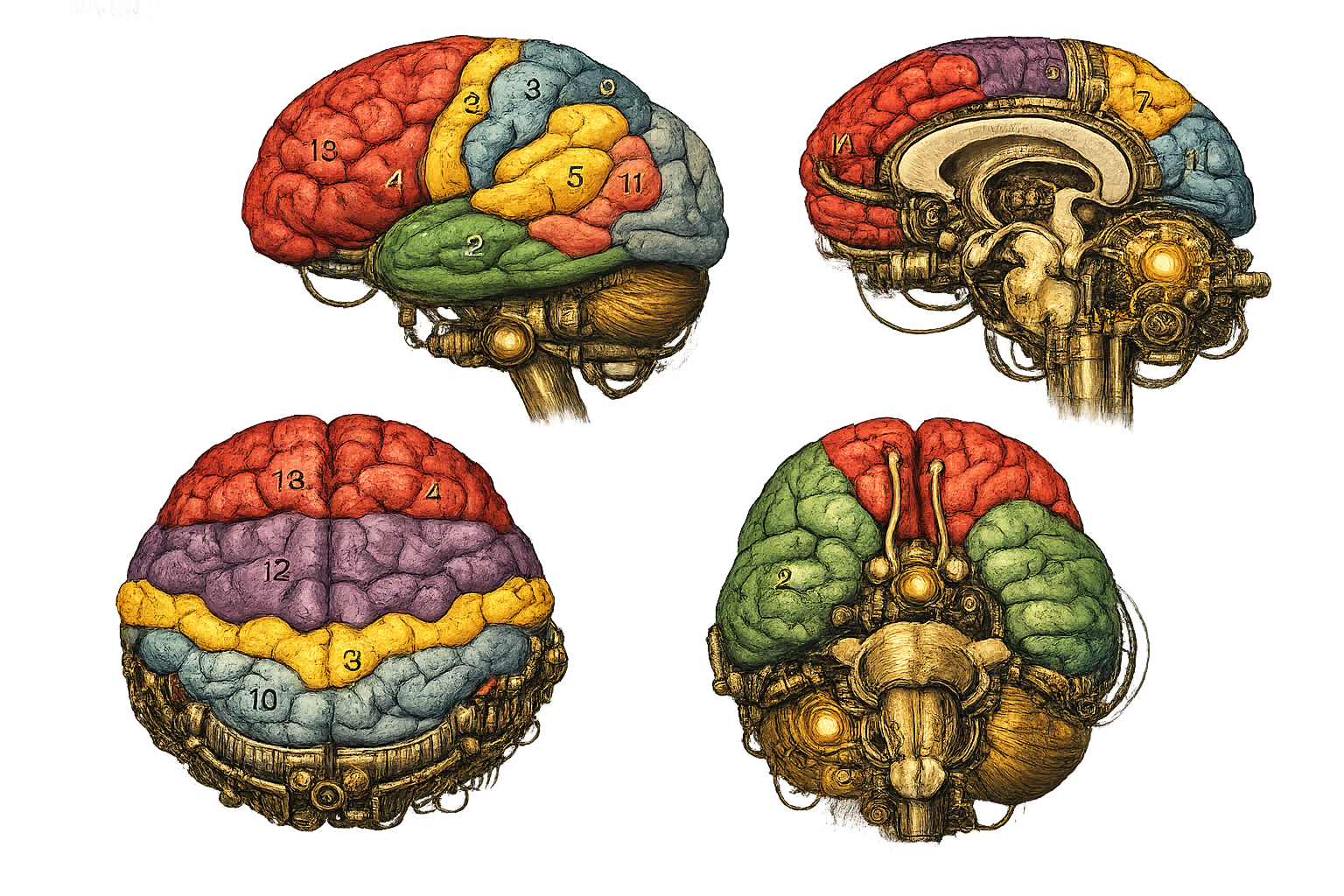
General intelligence doesn’t live in the motor cortex or the brainstem. The best neuroscience model we have for the “reasoning hardware” is the Parieto-Frontal Integration Theory (P-FIT), proposed by Jung & Haier (2007). P-FIT identifies a distributed network across the dorsolateral prefrontal cortex, anterior cingulate, and parietal association areas as the structural basis for general intelligence. It’s the hardware that does planning, abstraction, logical inference, and working memory.

To scale from the visual anchor to a reasoning estimate, I need three multipliers. Each one is genuinely uncertain, so I’ll give ranges rather than pretending I know the answer.

1. Volume Ratio

The P-FIT network is physically larger than the primary visual cortex. MRI volumetric studies put the ratio somewhere between 1.5× and 3×, depending on how generously you draw the boundaries.

Drawing boundaries in the brain is a lot like drawing boundaries on a map of the Middle East. Everyone has strong opinions, and nobody agrees.

Range: 1.5–3×. Central guess: ~2.25×

2. Computational Density

Not all neurons are equal. Pyramidal neurons in the prefrontal cortex have significantly more dendritic spines than neurons in V1, roughly 2–5× more synaptic connections per neuron, depending on layer and species. More spines means more integration per unit, which maps (loosely) to more parameters per computational element.

Range: 2–5×. Central guess: ~3×

3. Connectivity Overhead

Vision is architecturally local: a hierarchy of increasingly abstract feature detectors. Reasoning is architecturally global, requiring long-range white matter connections between distant brain regions. In transformer terms, it’s the difference between local attention and full self-attention. Long-range wiring is expensive.

How expensive? White matter tract studies suggest prefrontal regions have 1.25–2.5× the long-range connectivity density of sensory cortices.

Range: 1.25–2.5×. Central guess: ~1.75×

---

The Maths

From the Visual Anchor

Three multipliers, three ranges. Let’s see what falls out.

Low estimate (optimistic):

\[3.5\text{B} \times 1.5 \times 2.0 \times 1.25 = \mathbf{13.1\text{B}}\]

Central estimate:

\[3.5\text{B} \times 2.25 \times 3.0 \times 1.75 = \mathbf{41.3\text{B}}\]

High estimate (conservative):

\[3.5\text{B} \times 3.0 \times 5.0 \times 2.5 = \mathbf{131.3\text{B}}\]

Visual pathway range: 13B – 131B, central estimate ~41B.

From the Auditory Anchor

Now let’s run the same exercise starting from the ear instead of the eye. The multipliers are different because A1 and V1 have different architectures, so this is genuinely independent.

1. Volume ratio (5–12×, central ~8×). Primary auditory cortex (Heschl’s gyrus) is tiny — roughly 0.5–1.0 cm³, compared to V1’s ~5.4 cm³. The P-FIT network spans 5–12 cm³ of effective reasoning tissue, so the jump is much larger than from vision.

2. Computational density (1.5–3×, central ~2×). A1 has high neuron density (~68M/g) but lacks V1’s dominant spiny stellate population in layer 4 and has simpler synaptic machinery than prefrontal pyramidal neurons. The multiplier is smaller than for vision (2–5×) because the gap is narrower — A1 is already neuron-dense, just less synaptically complex.

3. Connectivity overhead (2–4×, central ~3×). A1 is strongly local: tonotopic organisation, ~400 μm horizontal processing spans. P-FIT requires extensive long-range tracts (SLF II, SLF III, arcuate fasciculus, callosal connections). Larger multiplier than vision (1.25–2.5×) because A1 is more locally wired than V1.

Low estimate:

\[1\text{B} \times 5 \times 1.5 \times 2 = \mathbf{15\text{B}}\]

Central estimate:

\[1\text{B} \times 8 \times 2 \times 3 = \mathbf{48\text{B}}\]

High estimate:

\[1\text{B} \times 12 \times 3 \times 4 = \mathbf{144\text{B}}\]

Auditory pathway range: 15B – 144B, central estimate ~48B.

Convergence

Two independent anchors. Different sensory modalities. Different multiplier profiles — vision starts from a larger cortical area with denser computation but less of a connectivity gap; audition starts from a much smaller area with a bigger volume jump but a smaller density correction. And yet:

	Low	Central	High
Visual anchor	13B	41B	131B
Auditory anchor	15B	48B	144B

The ranges overlap almost entirely. The central estimates differ by less than 20%. This is what you want from a Fermi estimate — robustness to anchor choice. If the answer depended heavily on which sensory system you started from, you’d worry. It doesn’t.

Combined range: ~13B to ~144B, with both central estimates landing in the 40–50B neighbourhood.

The spread is about one order of magnitude, which is par for the course with a Fermi estimate built on uncertain multipliers. The point isn’t the specific number. The point is what the range excludes.

It doesn’t include trillions.

---

What This Means (If It’s Even Roughly Right)

Both anchors point to the same neighbourhood: a 40–50B dense model, quantised to 4-bit, fits in about 20–25 GB of VRAM. That’s a single high-end consumer GPU. A 130–144B model at 4-bit needs ~65–72 GB, so a dual-GPU workstation or one professional card.

Current HBM3e already exceeds 1.5 TB/s bandwidth and the trend is steep. If reasoning-level AGI lives somewhere in this parameter range, the bottleneck isn’t memory or bandwidth. It’s architecture and training.

This also maps onto what we actually observe in practice, which is either encouraging or suspicious depending on your epistemological temperament. The 30–70B range is where open-weights models start to feel qualitatively different, where they go from “impressive autocomplete” to something that can sustain coherent multi-step reasoning. My own work on LLM Neuroanatomy found that models need a certain minimum size before their internal “reasoning circuits” cleanly separate from encoding and decoding functions. Below that critical mass, everything is entangled. Above it, genuine functional specialisation emerges.

That’s not proof of anything. But it’s consistent.

---

Where This Breaks Down

I should be honest about the many ways this could be garbage. In roughly descending order of how much they keep me up at night:

The anchors might be wrong. ASR isn’t hearing. Video understanding isn’t vision. If the “real” sensory compute floor is 10× higher than I’ve estimated, the whole thing shifts up an order of magnitude and we’re back to trillion-parameter territory. I don’t think that’s the case, because we often find out sensory models know a lot more than just what they were trained to do (like vision models building internal depth maps).

Reasoning might not scale from perception. The relationship between perceiving and thinking might not be a multiplicative scaling at all. Reasoning might require qualitatively different computational primitives: recursion, persistent state, learned search. Things that don’t map onto parameter count in any straightforward way. If that’s true, this entire approach is meaningless, and I’ve just done napkin maths for fun. (Which, honestly, is also fine. Note here that I fall into the more-was-better camp, a solid Mountcastlian (the theory that the entire cortex just scales up a single, universal algorithm)).

Transformers might be wildly more or less efficient than biology. The brain deals with noisy spiking neurons, slow chemical synapses, and a 20-watt power budget. Transformers have none of these constraints. Maybe a transformer parameter is “worth” 10 biological synapses. Maybe it’s worth 0.1. We genuinely don’t know. But I’m not arguing for Transformers, just the number of parameters.

Architecture matters enormously. A 50B transformer, a 50B state-space model, and a 50B hybrid with learned routing are three very different things. Parameter count alone is a terrible proxy for capability. The entire estimate assumes that “number of parameters” is a meaningful unit of comparison between biological and artificial systems, which is… optimistic. But it is at least a proxy for compute hardware.

Evolution doesn’t optimise for parameter efficiency. It optimises for survival. There could be massive redundancy in biological neural circuits: backup systems, evolutionary dead ends, dual-coding for robustness. None of that has an equivalent in a trained model. Biology might be over-provisioned by 10× for the reasoning task, in which case my biological multipliers are too high (directionally correct, based on my beer consumption at Uni).

---

The Takeaway

This is a thought experiment. I want to be clear about that. The multipliers are guesses. The anchors are approximations. The whole approach assumes a mapping between biological and artificial systems that might not hold.

But I think it’s a useful thought experiment, because it generates a number that’s much smaller than most people’s intuition.

When we think about AGI, we default to imagining something enormous. Elon’s space-based, planetary-scale compute. Trillions of parameters. Billion-dollar training runs. The Cortical Ratio suggests a different possibility: the minimum viable reasoning core might be surprisingly compact, and the “giant model” era might be a temporary consequence of architectural inefficiency rather than a fundamental requirement of the problem.

If even the conservative end of this estimate is in the right ballpark, AGI doesn’t need a data centre. It needs a better architecture.

We have the silicon. We’re waiting on the blueprint.

---

The “Cortical Ratio” is my name for this approach. It’s not established neuroscience terminology, just a useful framing. If you want to dig into the neuro side, Jung & Haier’s 2007 P-FIT paper is the starting point. For the compression trend in LLMs, the Qwen3.5 and Phi-4 technical reports are good recent data points.