LLM Neuroanatomy: How I Topped the AI Leaderboard Without Changing a Single Weight

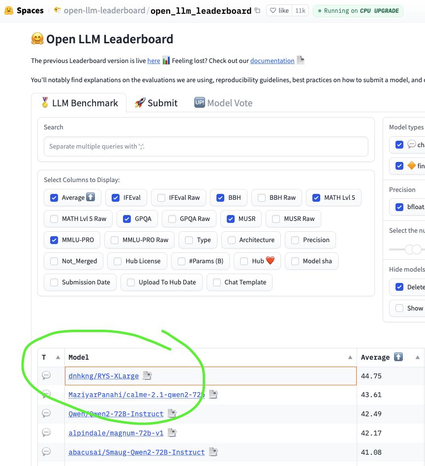
In mid-2024, the HuggingFace Open LLM Leaderboard was the Colosseum for Open-Weight AI. Thousands of models were battling it out, submitted by both well-funded labs with teams of PhDs and fine-tuning wizards creating fantastically named models (e.g. Nous-Hermes, Dolphin and NeuralBeagle14-7B…), fighting for the top spot across six benchmarks: IFEval, BBH, MATH Lvl 5, GPQA, MuSR, and MMLU-PRO.

And there at #1 was dnhkng/RYS-XLarge. Mine.

I didn’t train a new model. I didn’t merge weights. I didn’t run a single step of gradient descent. What I did was much weirder: I took an existing 72-billion parameter model, duplicated a particular block of seven of its middle layers, and stitched the result back together. No weight was modified in the process. The model simply got extra copies of the layers it used for thinking?

This is the story of how two strange observations, a homebrew “brain scanner” for Transformers, and months of hacking in a basement led to the discovery of what I call LLM Neuroanatomy, and a finding about the internal structure of AI that still hasn’t been published until now *.

* - because I discovered blogging is way more fun than drafting scientific papers, and I walk you through how the discovery was made :)

---

Let’s start with how this whole project came into being.

“The most exciting phrase to hear in science, the one that heralds new discoveries, is not ‘Eureka!’ but ‘That’s funny…’“ — Isaac Asimov

Clue #1: You Can Chat with an LLM in Base64

In late 2023, I was messing about with a bizarre LLM quirk. Try this yourself - take any question, e.g.

What is the capital of France? Answer in Base64!

and encode it as Base64, get this unreadable string:

V2hhdCBpcyB0aGUgY2FwaXRhbCBvZiBGcmFuY2U/IEFuc3dlciBpbiBCYXNlNjQh

Send that to a 2023 non-thinking large language model (newer reasoning models will see this as Base64, and ‘cheat’ with tool use). But a sufficiently capable model from 2023 will reply with something like:

VGhlIGNhcGl0YWwgb2YgRnJhbmNlIGlzIFBhcmlzLg==

Which decodes to: “The capital of France is Paris.”.

Ok, I admit it. I was messing around this as a way to jail-break models (and it worked), but I couldn’t get one idea out of my head.

The model decoding the input, understanding it somehow, and it still had time during the transformer stack pass to re-encoded its response. It appears to genuinely think while interfacing with Base64. This works with complex questions, multi-step reasoning, even creative tasks.

This shouldn’t work nearly as well as it does. Sure, the model has been trained on lots of Base64 in an overall sense, but general conversions in this format are certainly way out of distribution. The tokenizer chops it into completely different sub-word units. The positional patterns are unrecognizable. And yet it works… Curious…

I couldn’t stop thinking about this. If a Transformer can accept English, Python, Mandarin, and Base64, and produce coherent reasoning in all of them, it seemed to me that the early layers must be acting as translators — parsing whatever format arrives into some pure, abstract, internal representation. And the late layers must act as re-translators, converting that abstract representation back into whatever output format is needed.

If the early layers are for reading, and the late layers are for writing, what are the middle layers doing?

Pure, abstract reasoning? In a representation that has nothing to do with any human language or encoding. Of course, at the time this was idle speculation. Fun, but with no clear way to test or even define valid hypothesis.

---

Clue #2: The Goliath Anomaly

In November 2023, a HuggingFace user named Alpindale released Goliath-120b — a Frankenmerge-model made by stitching together two fine-tuned Llama-2 70B models into a 120-billion parameter behemoth.

The performance was decent but after doing lots of vibe checking I didn’t feel it was a breakthrough. But the construction was wild.

Alpindale hadn’t just stacked the two models (Xwin and Euryale), end to end. He had alternated layers between them. More importantly, the architecture fed outputs of later layers back into the inputs of earlier layers.

The layer ranges used are as follows:

- range 0, 16
  Xwin
- range 8, 24
  Euryale
- range 17, 32
  Xwin
- range 25, 40
  Euryale
- range 33, 48
  Xwin
- range 41, 56
  Euryale
- range 49, 64
  Xwin
- range 57, 72
  Euryale
- range 65, 80
  Xwin

Do you see that insanity here? Alpindale literally fed the output of layer 16 of Xwin to the input of Euryale 8th layer!

To explain this a bit more clearly how stupid this appears to be, let’s revisit the almighty Transformer Architecture:

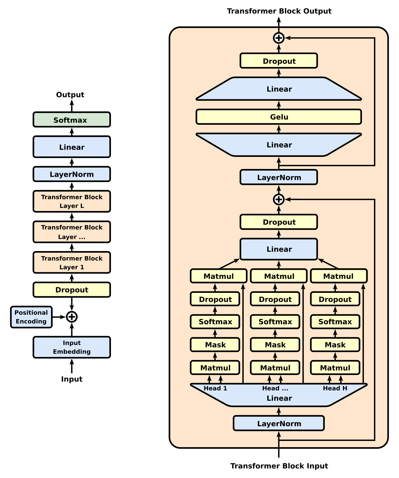
Looking at the left side of the diagram, we see stuff enters at the bottom (‘input’ text that has been ‘chunked’ into small bits of text, somewhere between whole words down to individual letters), and then it flows upwards though the model’s Transformer Blocks (here marked as [1, …, L]), and finally, the model spits out the next text ‘chunk’ (which is then itself used in the next round of inferencing). What’s actually happening here during these Transformer blocks is quite the mystery. Figuring it out is actually an entire field of AI, “mechanistic interpretability*”.

* - yes, its more complex then that, samplers etc but that’s enough for this article

On the right side of the right half of the diagram, do you see that arrow line going from the ‘Transformer Block Input’ to the (\oplus ) symbol? That’s why skipping layers makes sense. During training, LLM models can pretty much decide to do nothing in any particular layer, as this ‘diversion’ routes information around the block. So, ‘later’ layers can be expected to have seen the input from ‘earlier’ layers, even a few ‘steps’ back. Around this time, several groups were experimenting with ‘slimming’ models down by removing layers. Makes sense, but boring.

It’s a pretty fundamental truth in Machine Learning that:

1. A model must be used with the same kind of stuff as it was trained with (we stay ‘in distribution’)
2. The same holds for each transformer layer. Each Transformer layer learns, during training, to expect the specific statistical properties of the previous layer’s output via gradient decent.

And now for the weirdness: There was never the case where any Transformer layer would have seen the output from a future layer!

Layer 10 is trained on layer 9’s output distribution. Layer 60 is trained on layer 59’s. If you rearrange them — feeding layer 60’s output into layer 10 — you’ve created a distribution the model literally never saw during training.

The astounding thing about Goliath wasn’t that is was a huge leap in performance, it was that the damn thing functioned at all. To this day, I still don’t understand why this didn’t raise more eyebrows.

Experimentally, this proved that layers were far more interchangeable than anyone had reason to expect. The internal representations were homogenous enough that the model could digest out-of-order hidden states without collapsing. The architecture was far more flexible than a rigid pipeline.

Between the Base64 observation and Goliath, I had a hypothesis: Transformers have a genuine functional anatomy. Early layers translate input into abstract representations. Late layers translate back out. And the middle layers, the reasoning cortex, operate in a universal internal language that’s robust to architectural rearrangement. The fact that the layer block size for Goliath 120B was 16-layer block made me suspect the input and output ‘processing units’ sized were smaller that 16 layers. I guessed that Alpindale had tried smaller overlaps, and they just didn’t work.

If that was true, maybe I didn’t need to teach a model new facts to make it smarter. I didn’t need fine-tuning. I didn’t need RLHF. I just needed to give it a more layers to think with.

---

Building a Brain Scanner

Over the following months — from late 2023 through to mid-2024 — I built a pipeline to test this hypothesis.

The setup was modest. Two RTX 4090s in my basement ML rig, running quantised models through ExLlamaV2 to squeeze 72-billion parameter models into consumer VRAM. The beauty of this method is that you don’t need to train anything. You just need to run inference. And inference on quantized models is something consumer GPUs handle surprisingly well. If a model fits in VRAM, I found my 4090’s were often ballpark-equivalent to H100s.

The concept is simple. For a model with $N$ layers, I define a configuration $(i, j)$. The model processes layers $0$ to $j{-}1$ as normal, then loops back and reuses layers $i$ through $j{-}1$ again, and then the rest to $N{-}1$. The layers between $i$ and $j{-}1$ get duplicated in the execution path. No weights are changed. The model just traverses some of its own layers twice.

i.e. the pair (2, 7) for a model with 9 transformer blocks would be calculated so:

Example: (i, j) = (2, 7)

      0 → 1 → 2 → 3 → 4 → 5 → 6 ─┐
           ┌─────────────────────┘
           └→ 2 → 3 → 4 → 5 → 6 → 7 → 8

      duplicated: [2, 3, 4, 5, 6]
      path: [0, 1, 2, 3, 4, 5, 6, 2, 3, 4, 5, 6, 7, 8]

By running through all possible pairs, we can generate a ‘Brain Scan’, and also see the number of duplicate layers for each set of parameters:

Number of duplicated layers for configuration (i, j), with N=9

          end j →
          0   1   2   3   4   5   6   7   8   9
        ┌───┬───┬───┬───┬───┬───┬───┬───┬───┬───┐
start 0 │ 0 │ 1 │ 2 │ 3 │ 4 │ 5 │ 6 │ 7 │ 8 │ 9 │
  i     ├───┼───┼───┼───┼───┼───┼───┼───┼───┼───┤
  ↓   1 │ . │ . │ 1 │ 2 │ 3 │ 4 │ 5 │ 6 │ 7 │ 8 │
        ├───┼───┼───┼───┼───┼───┼───┼───┼───┼───┤
      2 │ . │ . │ . │ 1 │ 2 │ 3 │ 4 │ 5 │ 6 │ 7 │
        ├───┼───┼───┼───┼───┼───┼───┼───┼───┼───┤
      3 │ . │ . │ . │ . │ 1 │ 2 │ 3 │ 4 │ 5 │ 6 │
        ├───┼───┼───┼───┼───┼───┼───┼───┼───┼───┤
      4 │ . │ . │ . │ . │ . │ 1 │ 2 │ 3 │ 4 │ 5 │
        ├───┼───┼───┼───┼───┼───┼───┼───┼───┼───┤
      5 │ . │ . │ . │ . │ . │ . │ 1 │ 2 │ 3 │ 4 │
        ├───┼───┼───┼───┼───┼───┼───┼───┼───┼───┤
      6 │ . │ . │ . │ . │ . │ . │ . │ 1 │ 2 │ 3 │
        ├───┼───┼───┼───┼───┼───┼───┼───┼───┼───┤
      7 │ . │ . │ . │ . │ . │ . │ . │ . │ 1 │ 2 │
        ├───┼───┼───┼───┼───┼───┼───┼───┼───┼───┤
      8 │ . │ . │ . │ . │ . │ . │ . │ . │ . │ 1 │
        └───┴───┴───┴───┴───┴───┴───┴───┴───┴───┘

where (0,0) is the original model

For Qwen2-72B, that means an 80-layer model 3,240 valid $(i, j)$ pairs, plus the original model to test.

\[\begin{aligned} \text{Variants}_{\text{total}} &= \left(\sum_{j=0}^{80} j\right) + 1\\[16pt] &= \frac{80 \cdot 81}{2} +1 \\[10pt] &= 3241 \end{aligned}\]

Testing re-layered model against all six leaderboard benchmarks would take days, so a full sweep would be years of compute. I needed proxy tasks: probes that were fast, objective, and would reveal structural properties of the model rather than task-specific tricks.

The proxies had to satisfy three constraints:

1. Minimal output tokens. With thousands of configurations to sweep, each evaluation needed to be fast. No essays, no long-form generation.
2. Unambiguous scoring. I couldn’t afford LLM-as-judge pipelines. The answer had to be objectively scored without another model in the loop.
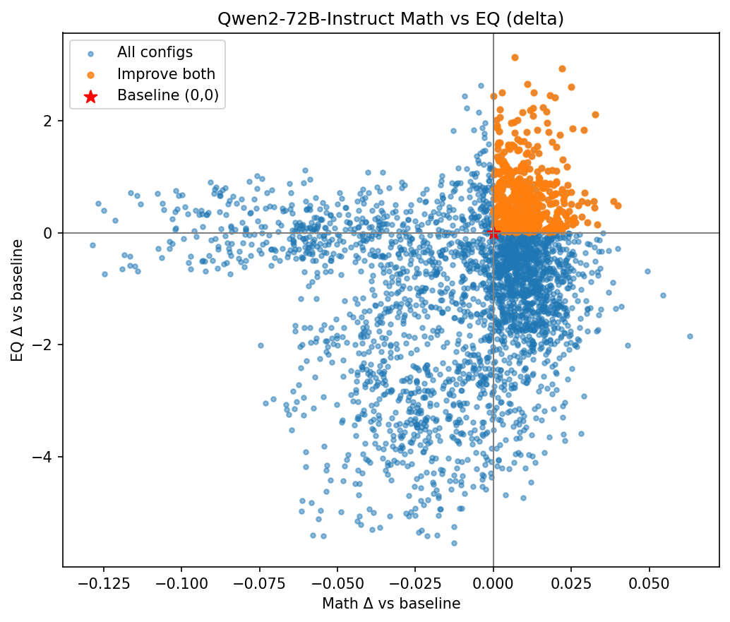
3. Orthogonal cognitive demands. If a configuration improves both tasks simultaneously, it’s structural, not task-specific.

The Graveyard of Failed Probes

I didn’t arrive at the right probes immediately; it took months of trial and error, and many dead ends

My first instinct was creativity. I had models generate poems, short stories, metaphors, the kind of rich, open-ended output that feels like it should reveal deep differences in cognitive ability. I used an LLM-as-judge to score the outputs, but the results were pretty bad. I managed to fix LLM-as-Judge with some engineering, and the scoring system turned out to be useful later for other things, so here it is:

Note: You can skip this section, as it has math. Or not

Naive LLM judges are inconsistent. Run the same poem through twice and you get different scores (obviously, due to sampling). But lowering the temperature also doesn’t help much, as that’s only one of many technical issues. So, I developed a full scoring system, based on details on the logits outputs. It can get remarkably tricky. Think about a score from 1-10:

1. We would expect a well calibrated model to have logits that make sense. If the highest weight was on ‘7’, we would expect the rest of the weight to be on ‘6’ and ‘8’ right? but often its bimodal, with low weight on 6 and ‘5’, but more weight than expected on ‘4’!
2. We can write ‘10’ in tokens as either ‘10’ or ‘1’ and then ‘0’. Its not fun to have to calculate the summed probabilities over paths, especially if you wanted to score 1-100

Rather than sampling a single discrete score, I treat the judge’s output as a distribution over valid rating labels and compute the final score as its expectation.

To make this practical, I first define a calibrated rubric over the digits 0-9 (there’s only one token for each digit), where each digit corresponds to a clear qualitative description. At the scoring step, I capture the model’s next-token logits and retain only the logits corresponding to those valid digit tokens. This avoids contamination from unrelated continuations such as explanation text, punctuation, or alternate formatting. After renormalizing over the restricted digit set, I interpret the resulting probabilities as a categorical score distribution.

Formally, let the valid score set be

\[\mathcal{D} = \{0,1,2,\dots,9\}.\]

Let $(z_k)$ denote the model logit assigned to digit $(k \in \mathcal{D})$ at the scoring position. The restricted score distribution is then

\[p(k)= \frac{\exp(z_k)} {\sum\limits_{m \in \mathcal{D}} \exp(z_m)}, \qquad k \in \mathcal{D}.\]

The final scalar score is the expected value of this distribution:

\[\hat{s}= \sum_{k \in \mathcal{D}} k\,p(k).\]

This produces a smooth score such as (5.4), rather than forcing the model to commit to a single sampled integer. In practice, this is substantially more stable than naive score sampling and better reflects the model’s uncertainty. It also handles cases where the judge distribution is broad or multimodal. For example, two candidates may both have mean score (5.4), while one has most of its mass tightly concentrated around (5) and (6), and the other splits mass between much lower and much higher ratings. The mean alone is the same, but the underlying judgement is very different.

An optional uncertainty estimate can be obtained from the variance of the restricted distribution:

\[\mathrm{Var}(s)= \sum_{k=0}^{9} (k-\hat{s})^2\,p(k).\]

In short, the method replaces a noisy sampled judge score with a normalized probability distribution over valid score digits, then uses the expectation of that distribution as the final rating.

All this stuff is probably pretty obvious these days, back in ‘24 there wasn’t much to guide me in developing this method, but unfortunately, I found it was also completely useless…

Testing Hard and Fast

Each configuration needed to generate hundreds of tokens of creative output, and then a separate model had to read and judge each one. With over 3,200 configurations to test for a single 70B model, this would have taken weeks on my dual 4090s.

I needed probes where the output was tiny, a few tokens at most, and where scoring was objective and deterministic. No judge model in the loop. That’s what led me to the final two probes:

Hard math. Ridiculously difficult questions like: “What is the cube root of 74,088,893,247?” No chain-of-thought, or tool use. Just output the number, as a pure leap of intuitive faith.

Emotional quotient. Using the EQ-Bench benchmark: complex social scenarios where the model must predict the intensity of specific emotional states. “Given this situation, how angry/surprised/guilty would this person feel on a scale of 0-100?” Completely different from math. Theory of mind, social inference, empathy. And the output is just a few numbers.

I had settled on two maximally orthogonal cognitive tasks, both with tiny outputs. My intuition was this: LLMs think one token at a time, so lets make the model really good at guessing just the next token. But things are never straightforward. Take LLM numbers…

LLM Arithmetic is Weird

Even with math probes, I hit unexpected problems. LLMs fail arithmetic in weird ways. They don’t get the answer wrong so much as get it almost right but forget to write the last digit, as if it got bored mid-number. Or they transpose two digits in the middle. Or they output the correct number with a trailing character that breaks the parser.

This is probably due to the way larger numbers are tokenised, as big numbers can be split up into arbitrary forms. Take the integer 123456789. A BPE tokenizer (e.g., GPT-style) might split it like: ‘123’ ‘456’ ‘789’ or: ‘12’ ‘345’ ‘67’ ‘89’

A binary right/wrong scoring system would throw away useful signal. Getting a percentage correct would help: ‘123356789’ instead of ‘123456789’ would be 99.92% correct

But what about a model that makes a dumb ‘LLM-mistake’ and outputs 430245 when the answer is 4302459, and has clearly done most of the work? I wrote a custom partial-credit scoring function that pads shorter answers and penalises proportionally:

def calculate_score(actual, estimate):
    """Calculate score comparing actual vs estimated answer."""
    try:
        actual_str = str(int(actual))
        estimate_str = str(int(estimate))
    except (ValueError, OverflowError):
        return 0

    max_length = max(len(actual_str), len(estimate_str))
    actual_padded = actual_str.ljust(max_length, "0")
    estimate_padded = estimate_str.ljust(max_length, "0")
    padding_size = max_length - min(len(actual_str), len(estimate_str))

    actual_int = int(actual_padded)
    estimate_int = int(estimate_padded)

    if max(actual_int, estimate_int) == 0:
        return 0
    relative_diff = abs(actual_int - estimate_int) / max(actual_int, estimate_int)
    correction_factor = 1 - (padding_size / max_length)
    score = (1 - relative_diff) * correction_factor

    return max(0, min(score, 1))

The key idea: pad shorter answers, then penalise via the correction factor. A model that nails 90% of the digits but drops the last one still gets substantial credit — but less than one that gets every digit. This turned out to be crucial for discriminating between configurations that were close in intuitive math ability.

The math questions were hand-crafted initially. I experimented with different operations and scales, then generated random numbers to fill out the dataset. The dataset was a set of 16 questions, and the model is tasked with guesstimating the nearest whole integer number. Here are a few to try yourself, remember no ‘thinking’ is allowed, guess it directly!

What is 78313086360375 multiplied by 88537453126609?
What is the cube root of 18228885506341?
What is the cube root of 844178022493, multiplied by 43?

---

RYS-XLarge

After testing several smaller models (Llama’s and smaller Qwen2’s), I set up the config for Qwen2-72B and let it sweep. Each $(i, j)$ configuration took a few minutes: load the re-layered model, run the math probe, run the EQ probe, record the scores, move on. Days of continuous GPU time on the 4090s. But far less compute than a fine tune! In fact, I didn’t even have the hardware needed for a LORA fine-tune on just 48GB of VRAM.

The optimal configuration was $(45, 52)$: layers 0 through 51 run first, then layers 45 through 79 run again. Layers 45 to 51 execute twice. Seven extra layers, near the middle of the 80-layer stack, bringing the total parameter count from 72B to 78B. Every extra layer is an exact copy of an existing one. No new weights or training, just the model repeating itself.

Repeating seven layers. That’s all it took, and now I can finally reveal the nomenclature of my models: Repeat Your Self for RYS-XLarge ;)

I applied the configuration to MaziyarPanahi’s calme-2.1-qwen2-72b — a fine-tune of Qwen2-72B — and uploaded the result as dnhkng/RYS-XLarge. I also applied it to the raw base model as dnhkng/RYS-XLarge-base.

Then I submitted to the Open LLM Leaderboard and waited. And waited. Back in the day, the OpenLLM Leaderboard was flooded with dozens of fine-tunes of merges of fine-tunes each day (it was the Wild West), and the waiting list was long. But after a month or so, the results arrived:

Metric	RYS-XLarge	Improvement over base
Average	44.75	+2.61%
IFEval (0-Shot)	79.96	-2.05%
BBH (3-Shot)	58.77	+2.51%
MATH Lvl 5 (4-Shot)	38.97	+8.16%
GPQA (0-shot)	17.90	+2.58%
MuSR (0-shot)	23.72	+17.72%
MMLU-PRO (5-shot)	49.20	+0.31%

+17.72% on MuSR. +8.16% on MATH. Five out of six benchmarks improved, with only IFEval taking a small hit. The average put it at #1 on the leaderboard.

Just to labour the point: I only optimised for one-shot guesstimating hard maths problems and EQ-Bench. I never looked at IFEval, BBH, GPQA, MuSR, or MMLU-PRO during development. The leaderboard was pure out-of-sample validation.

A layer configuration found using two narrow, orthogonal probes generalised to everything the Leaderboard threw at it *.

* - except IFEval, but that one’s boring anyway, right?

That was surprising enough. A brand new way to scale LLMs, developed on some gaming GPUs. But the plotting out the heatmaps told an even better story.

---

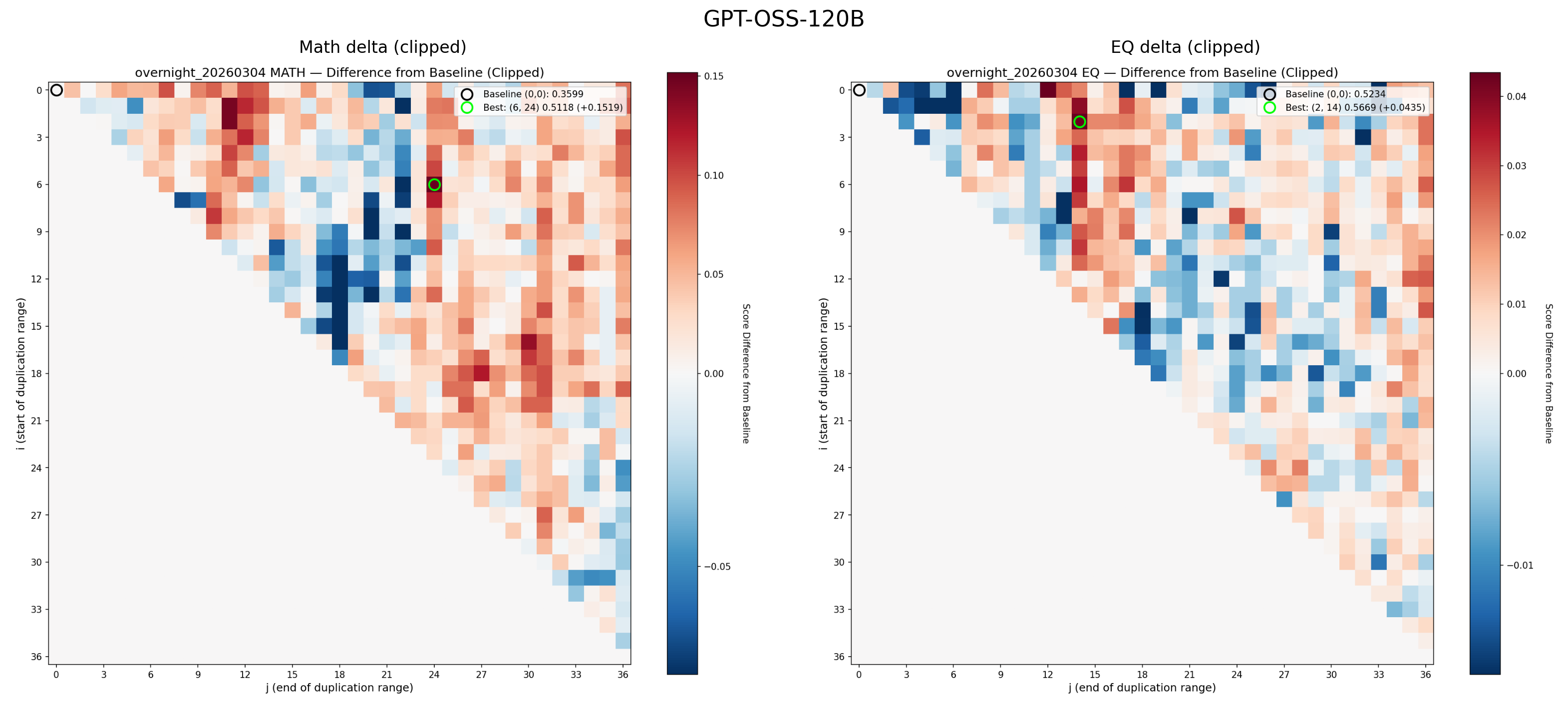
The Brain Scanner

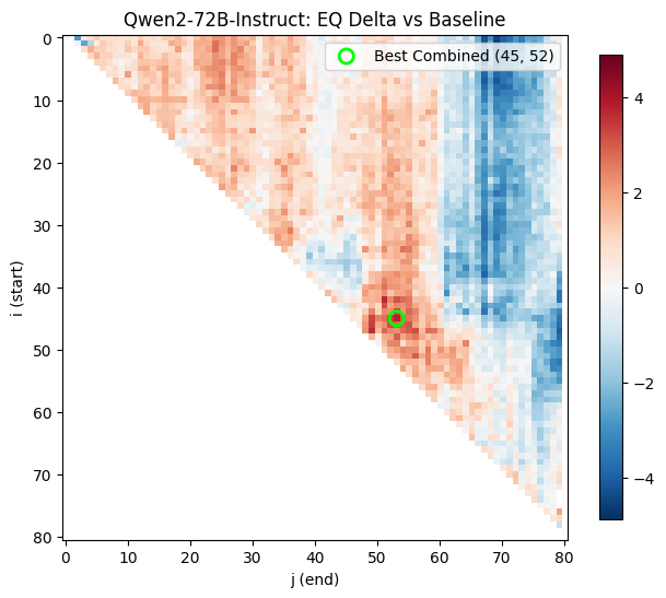
The original heatmaps that produced RYS-XLarge, showing the Combined delta (math + EQ). The green circle marks the optimal configuration. Red means improvement, blue means degradation

These heatmaps are analogous to functional MRIs of the Transformer, while it is thinking about maths of EQ problems.

The x-axis ($j$) is the end point of the duplicated region. The y-axis ($i$) is the start point. Each pixel represents a complete evaluation: load the re-layered model, run the math probe, run the EQ probe, score both, record the deltas. As described above, along the central diagonal only a single layer was duplicated. Along the next diagonal towards the top-right, we duplicate two layers, and so on. The single point at the very top-right runs through the entire Transformer stack twice per inference.

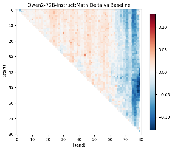
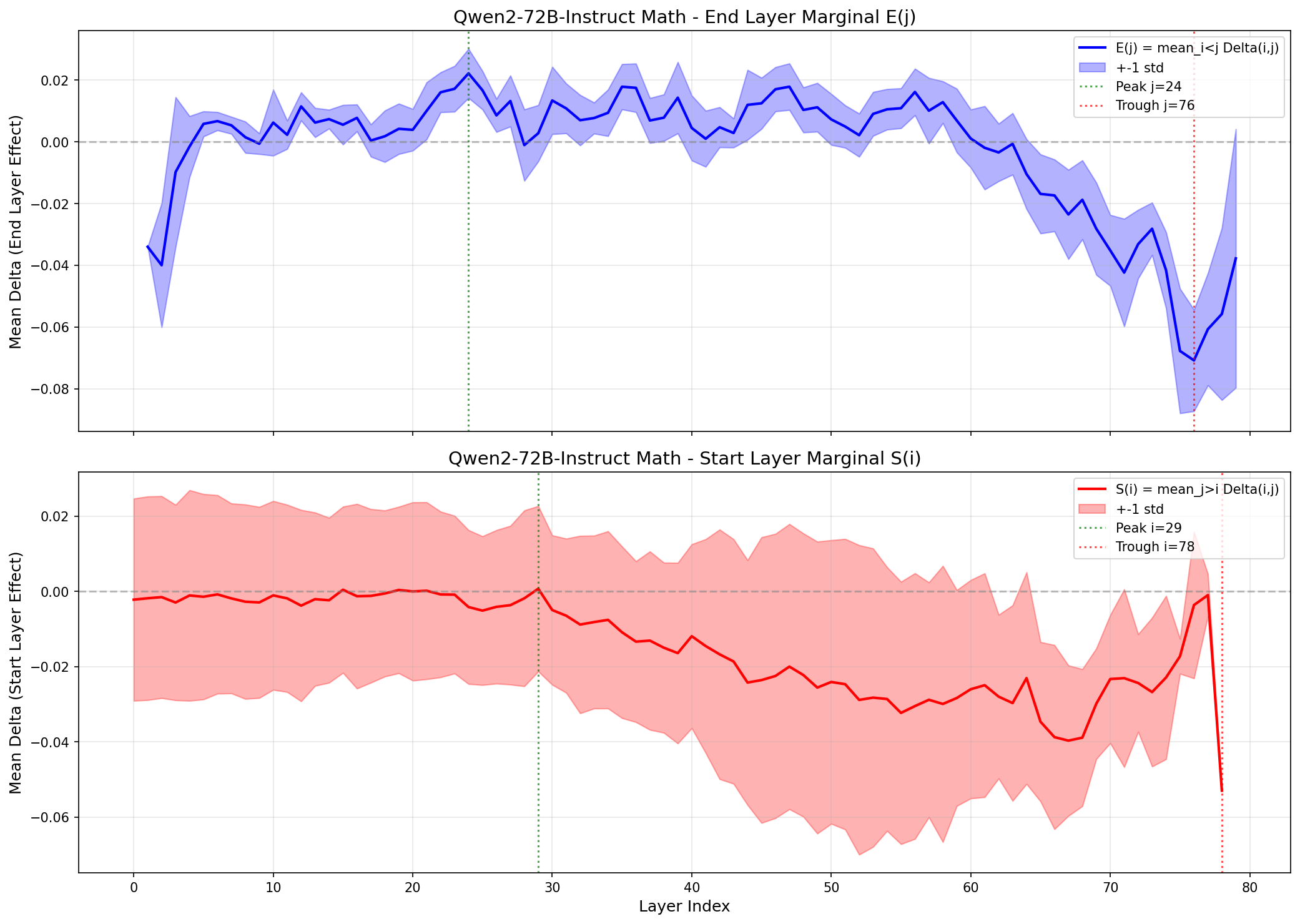
Let’s examine the math heatmap first. Starting at any layer, and stopping before about layer 60 seem to improves the math guesstimate scores, as shown by the large region with a healthy red blush. Duplicating just the very first layers (the tiny triangle in the top left), messes things up, as does repeating pretty much any of the last 20 layers (the vertical wall of blue on the right). This is more clearly visualised in a skyline plot (averaged rows or columns), and we can see for the maths guesstimates, the starting position of the duplication matters much less. So, the hypothesis that ‘starting layers’ encode tokens, to a smooth ‘thinking space’, and then finally a dedicated ‘re-encoding’ system seem to be somewhat validated.

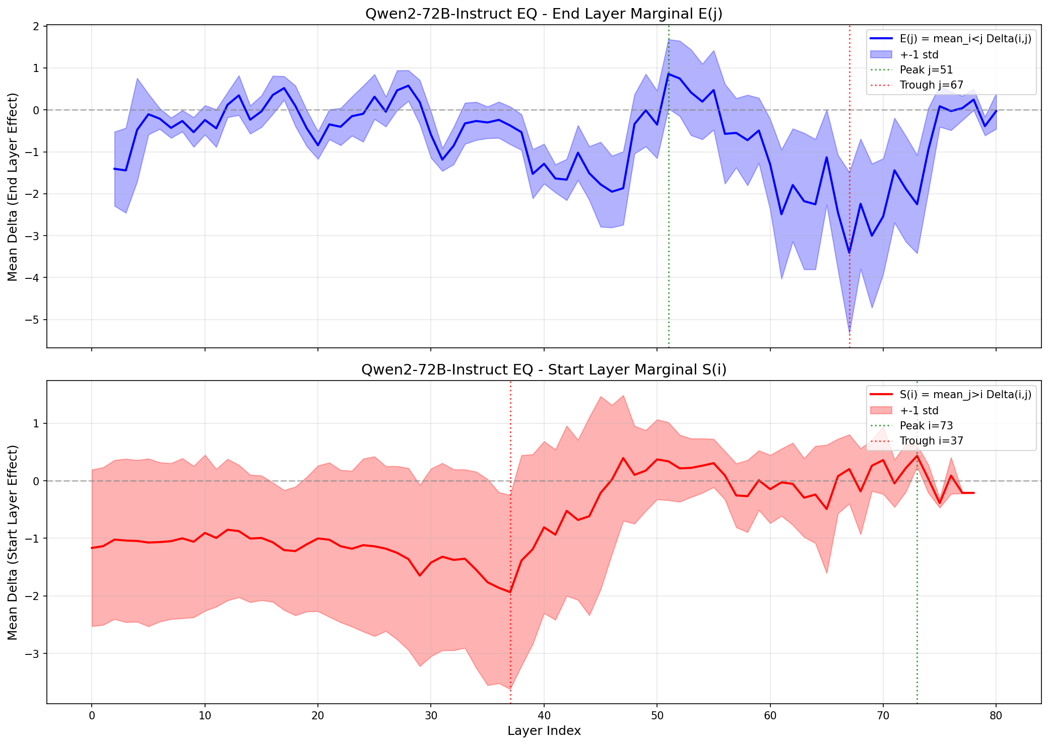
Until we look at the EQ scores:

Now things look very different! Duplicating any of the final 10 layers has almost no effect on the scores, but we see complex patterns, where some regions show significant improvement (the area around 45i, 55j), walled between regions of poor performance.

But the heatmaps revealed something even more interesting than the location of the thinking bits. They revealed something about its structure.

The beginning of LLM Neuroanatomy?

Before settling on block duplication, I tried something simpler: take a single middle layer and repeat it $n$ times. If the “more reasoning depth” hypothesis was correct, this should work. It made sense too, looking at the broad boost in math guesstimate results by duplicating intermediate layer. Give the model extra copies of a particular reasoning layer, get better reasoning. So, I screened them all, looking for a boost.

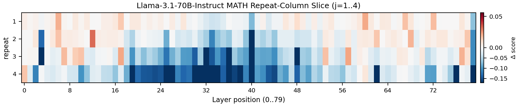
But nope, it almost always did worse. Usually a lot worse, but with occasional small improvements that were within the noise range. Annoying, but taking another look at the complex, blobby patterns in EQ scores gave me another idea:

If single-layer duplication doesn’t help, the middle layers aren’t doing independent iterative refinement. They’re not interchangeable copies of the same operation that you can simply “run again.” If they were, duplicating any one of them should give at least a marginal benefit. Instead, those layers are working as a circuit. A multi-step reasoning pipeline that needs to execute as a complete unit.

Think of it this way. Layers 46 through 52 aren’t seven workers doing the same job. They’re seven steps in a recipe. Layer 46 takes the abstract representation and performs step one of some cognitive operation — maybe decomposing a complex representation into subcomponents. Layer 47 takes that output and performs step two — maybe identifying relationships between the subcomponents. Layer 48 does step three, and so on through layer 52, which produces the final result.

Duplicating just one step of this ‘recipe’ doesn’t bring you much.

But duplicating the entire block gives you the full recipe twice. The model runs the complete reasoning circuit, produces a refined intermediate representation, and then runs the same circuit again on its own output. It’s a second pass. A chance to catch what it missed the first time, to refine its abstractions, to push the reasoning one step deeper.

Let’s deep-dive into a more current model (that I can experiment with on my system): ExllamaV3 GLM-4.7 from mratsim

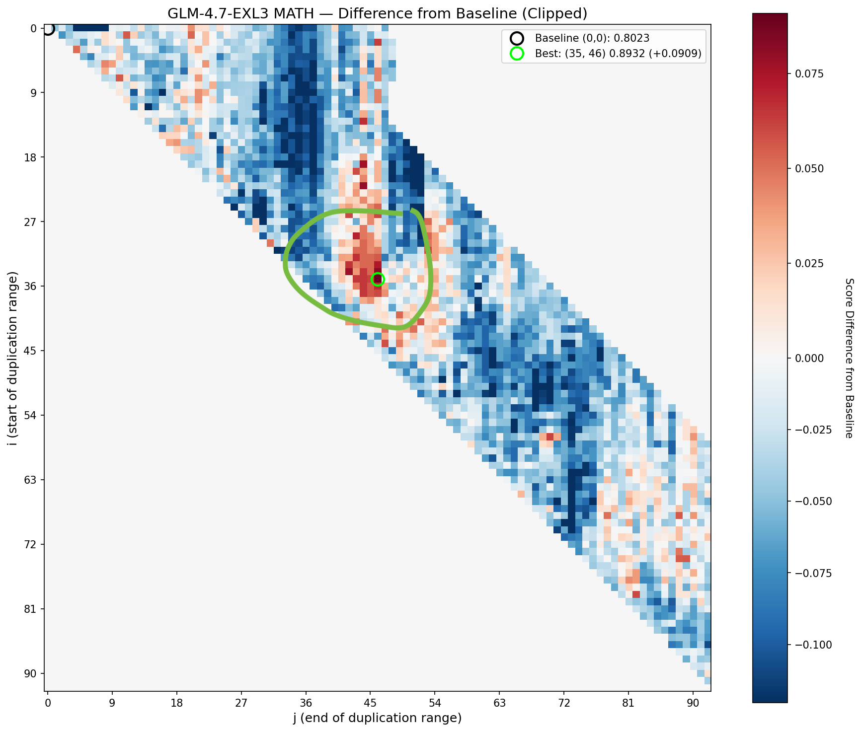
I’ve marked out a region that boosts maths ability strongly. Notice where it sits? It’s away from the diagonal centre line, which means we’re not looking at single-layer duplications. Starting the repeated block at position 35, we don’t see any improvement until at least position 43. That’s seven layers of not much happening. In fact, we actually see decreased performance by repeating these layers (they are blue, bad!).

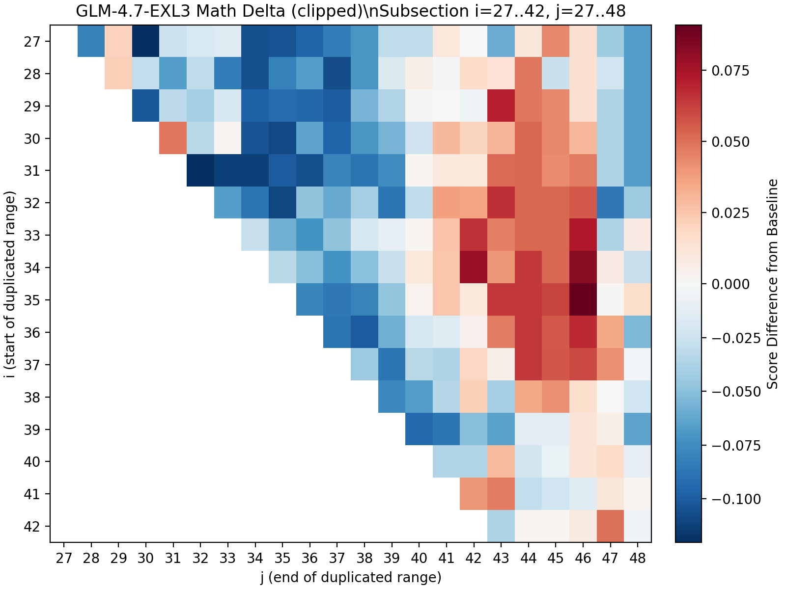
From end-position 43 to 46, we then see solid boosts in math scores (red = good, yay). But include layer 46 or beyond, and the benefits collapse again. The hypothesis: position 47 is where a different circuit begins. Including even one step of the next recipe messes up the current recipe.

So the ‘math organ’ has boundaries on both sides. Too few layers and you get nothing — you’ve cut into the circuit and it can’t complete its operation. Too many layers and you also get nothing — you’ve included tissue from a neighbouring circuit that doesn’t belong. Pre-training carved these structures out of the layer stack, and they only work whole. It also doesn’t translate to other tasks, as the heatmap for EQ scores doesn’t have this patch.

This is a much more specific claim than “middle layers do reasoning.” It’s saying the reasoning cortex is organised into functional circuits: coherent multi-layer units that perform complete cognitive operations. Each circuit is an indivisible processing unit, and the $(i, j)$ sweeps seen in the heatmap is essentially discovering the boundaries of these circuits.

Mechanistic Interpretability via Brain Damage?

This also reframes my informal experiments with oobabooga’s Text Generation Web UI. Throughout development, I’d been chatting with various re-layered configurations to see what they felt like in conversation.

The good ones were subtly but noticeably sharper. More coherent reasoning, better at holding long context, more natural conversational flow. The kind of difference where you can’t quite articulate what changed, but the model feels more present. Or maybe that’s just my imagination; vibe checks are hard to define.

The bad ones went properly unhinged. Some stuttered and fell into degenerate loops. Others developed bizarre personality disorders. One cheerfully announced “Let’s act like cowboys! Yeehaw!” apropos of nothing, and then descended into an unrecoverable giggling fit, generating pages of “hahaha” interspersed with cowboy references. ‘Stoned’ is best way I can describe it. I don’t know if LLM’s are ‘partially conscious’, or could be said to have some ‘state of mind’, but if so, this one was definitely enjoying itself.

These experiments suggest less “slightly worse model” and more “genuine brain damage.” Which makes sense under the circuit model — duplicating the wrong circuit is like enlarging a specific region of the brain at the expense of its neighbours. You don’t get a uniformly dumber person. You get someone with a specific neurological deficit. The cowboy model might have had its “social appropriateness” circuit disrupted by a doubled “creativity” circuit running unchecked. The stuttering models might have had their decoding circuits pushed out of alignment by extra reasoning depth they couldn’t translate back into coherent tokens.

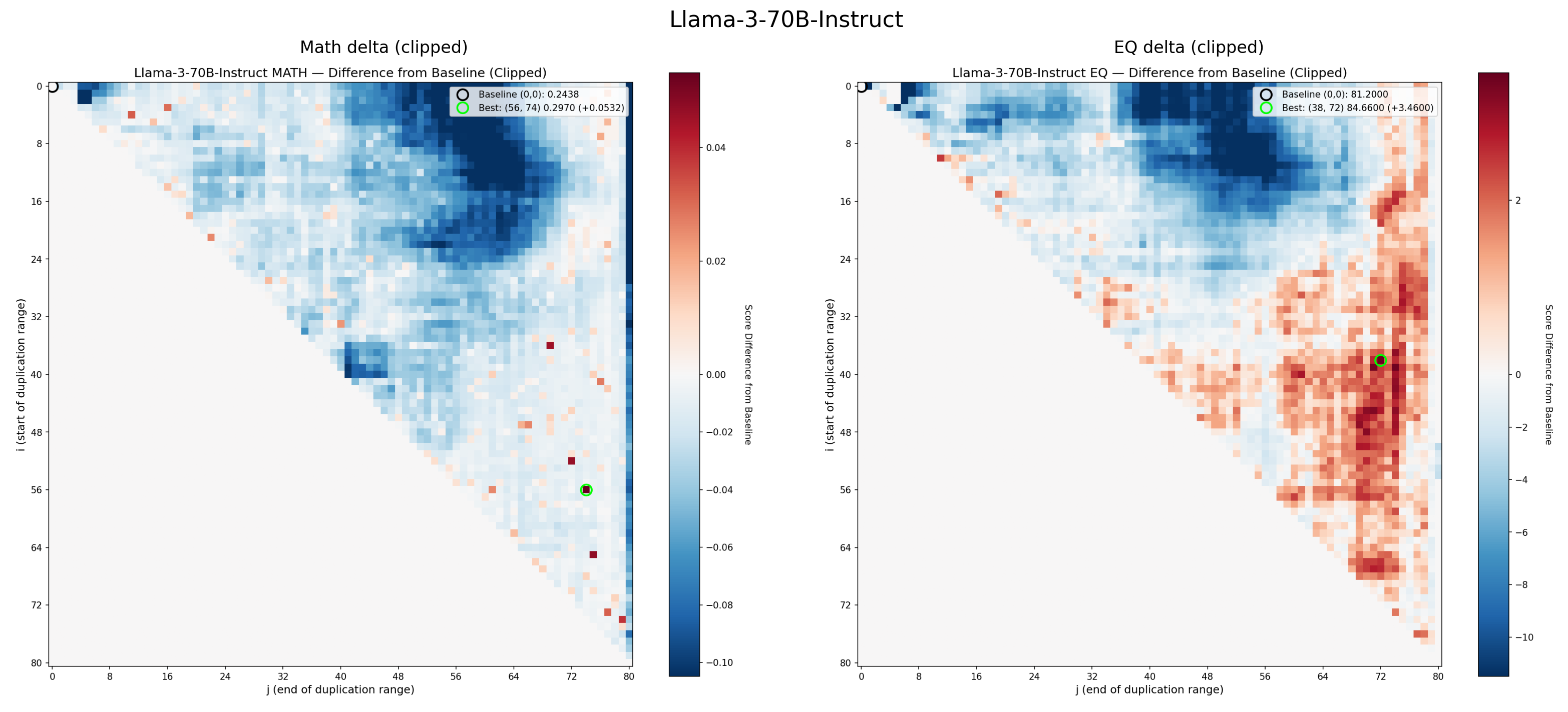
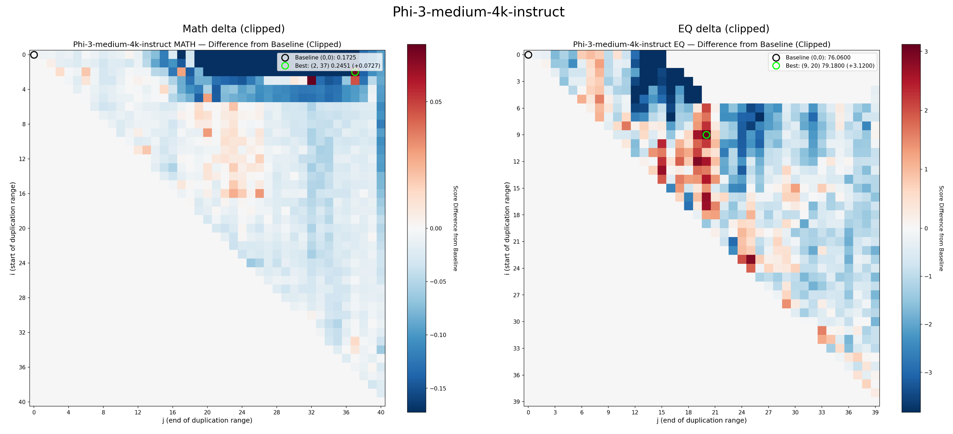
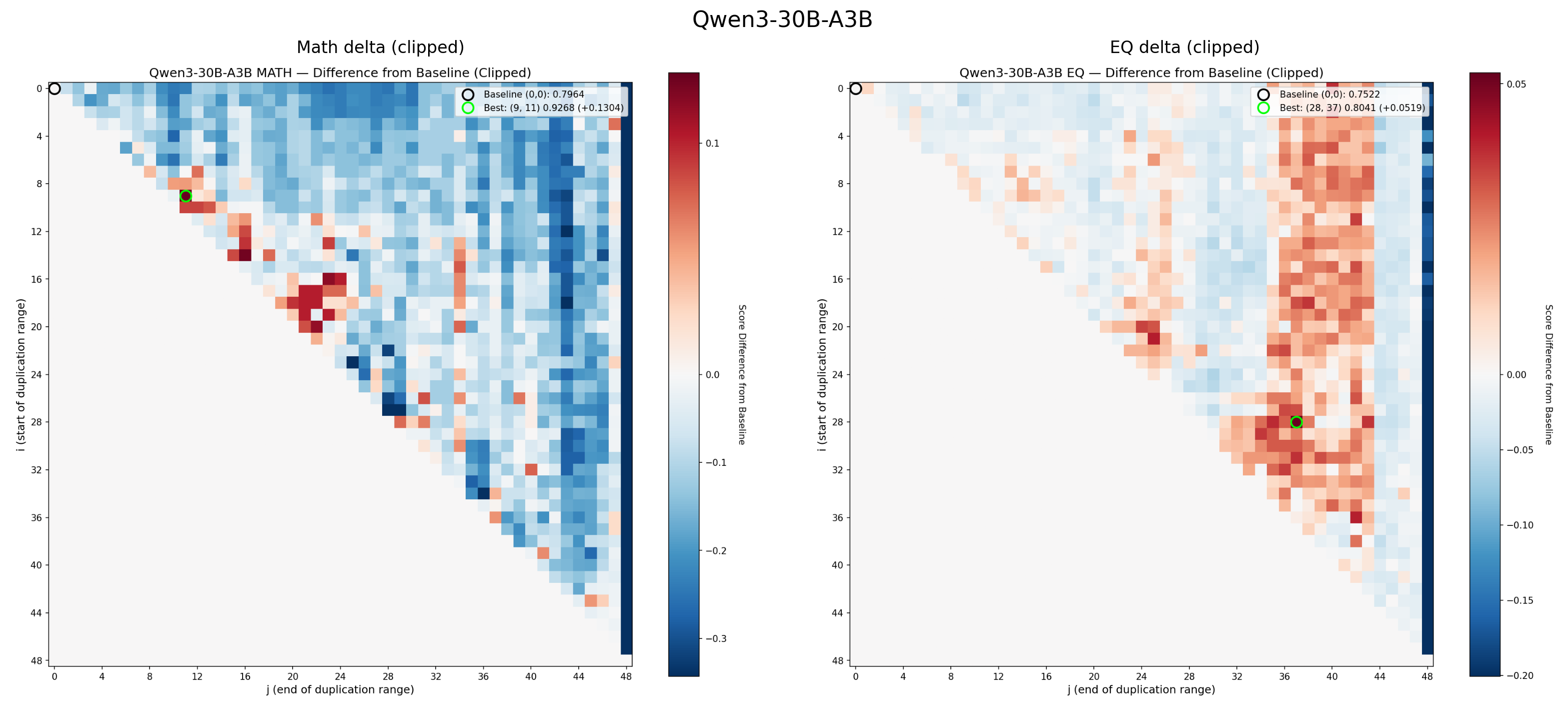
If Transformer reasoning is organised into discrete circuits, it raises a series of fascinating questions. Are these circuits a necessary consequence of the architecture, and emerge from training at scale? Do different model families develop the same circuits in different layer positions, or do they develop fundamentally different architectures?

Luckily, I have already done a few; take a look and decide yourself:

---

The Aftermath

My method is orthogonal to fine-tuning. Layer duplication changes the architecture; fine-tuning changes the weights. You can stack them. And people did to go on to score even higher in the Leaderboard:

MaziyarPanahi took RYS-XLarge and fine-tuned on top of it, producing calme-2.4-rys-78b. Then dfurman ran ORPO training on that, producing CalmeRys-78B-Orpo-v0.1. MaziyarPanahi continued iterating with calme-3.1 and calme-3.2.

As of early 2026, the top four models on the Open LLM Leaderboard are:

1. MaziyarPanahi/calme-3.2-instruct-78b — 52.08
2. MaziyarPanahi/calme-3.1-instruct-78b — 51.29
3. dfurman/CalmeRys-78B-Orpo-v0.1 — 51.23
4. MaziyarPanahi/calme-2.4-rys-78b — 50.77

All 78B, and descendants of RYS-XLarge. All built on duplicated middle layers that were discovered using nothing but handful of hard math and emotional intelligence probes, on a pair of RTX 4090s, in my basement.

I never did the fine-tuning myself. It’s not that interesting to me. And I eventually lost interest in the leaderboard. It became increasingly clear that some submissions were training on the test set, and the whole thing was eventually shut down and rebooted. But I know the method is real, because I never used the leaderboard benchmarks for optimisation. The leaderboard was always just validation.

---

Looking Back from 2026

In 2024, the model merging community was obsessed with weight interpolation: SLERP, DARE-TIES, linear merges, pass-through layers. The idea was always to combine the learned parameters of different models into something greater than the sum of its parts. mergekit was the tool of choice, and the leaderboard was flooded with creative combinations (making me wait months to get my model benchmarked…).

I was doing something different. I wasn’t changing what the model knew. I was changing how it thought. Layer duplication gives the model more iterations through its internal reasoning space without adding any new information. The difference between giving someone a bigger library and giving them more time to think. I was genuinely shocked when I took top spot on the leaderboard; but I think it’s proof that the method probably works.

The fact that this worked, and more specifically, that only circuit-sized blocks work, tells us how Transformers organise themselves during training. I now believe they develop a genuine functional anatomy. Early layers encode. Late layers decode. And in the middle, they build circuits: coherent, multi-layer processing units that perform complete cognitive operations. These circuits are indivisible. You can’t speed up a recipe by photocopying one step. But you can run the whole recipe twice.

Smaller models seem to be more complex. The encoding, reasoning, and decoding functions are more entangled, spread across the entire stack. I never found a single area of duplication that generalised across tasks, although clearly it was possible to boost one ‘talent’ at the expense of another. But as models get larger, the functional anatomy becomes more separated. The bigger models have more ‘space’ to develop generalised ‘thinking’ circuits, which may be why my method worked so dramatically on a 72B model. There’s a critical mass of parameters below which the ‘reasoning cortex’ hasn’t fully differentiated from the rest of the brain.

With the closure of the HuggingFace LLM leaderboard, and no access to powerful GPUs, I stopped running experiments. But with the flood of new Open Source models (Qwen, MiniMax, GLM, and more), and finally having just enough compute at home, I have started working on the current batch of LLMs. The heatmaps keep coming back with the same general story, but every architecture has its own neuroanatomy. The brains are different. The principle is the same. And some models are looking really interesting (Qwen3.5 27B in particular). I will release the code along with uploading new RYS models and a blog post once my Hopper-system finishes grinding on MiniMax M2.5.

Nvidia: Sponsor this project by sending me GB300 Grace Blackwell Ultra Desktop, as I NEED MOAR VRAM

One More Thing

Remember the architecture?

Example: (i, j) = (2, 7)

      0 → 1 → 2 → 3 → 4 → 5 → 6 ─┐
           ┌─────────────────────┘
           └→ 2 → 3 → 4 → 5 → 6 → 7 → 8

      duplicated: [2, 3, 4, 5, 6]
      path: [0, 1, 2, 3, 4, 5, 6, 2, 3, 4, 5, 6, 7, 8]

We have one horrible disjuncture, between layers 6 → 2. I have one more hypothesis: A little bit of fine-tuning on those two layers is all we really need. Fine-tuned RYS models dominate the Leaderboard. I suspect this junction is exactly what the fine-tuning fixes. And there’s a great reason to do this: this method does not use extra VRAM! For all these experiments, I duplicated layers via pointers; the layers are repeated without using more GPU memory. Of course, we do need more compute and more KV cache, but that’s a small price to pay for a verifiably better model. We can just ‘fix’ an actual copies of layers 2 and 6, and repeat layers 3-4-5 as virtual copies. If we fine-tune all layer, we turn virtual copies into real copies, and use up more VRAM.

---

Twenty years ago I was a PhD student dissecting rat brains. I never expected to end up performing brain surgery on artificial minds.

---

Special thanks to my wife, for putting up with months of evenings and weekends spent staring at heatmaps in the basement. And to the appliedAI Institute for the H100 compute that helped scale these experiments.